Note
This tutorial was generated from an IPython notebook that can be downloaded here.
PSD Normalization
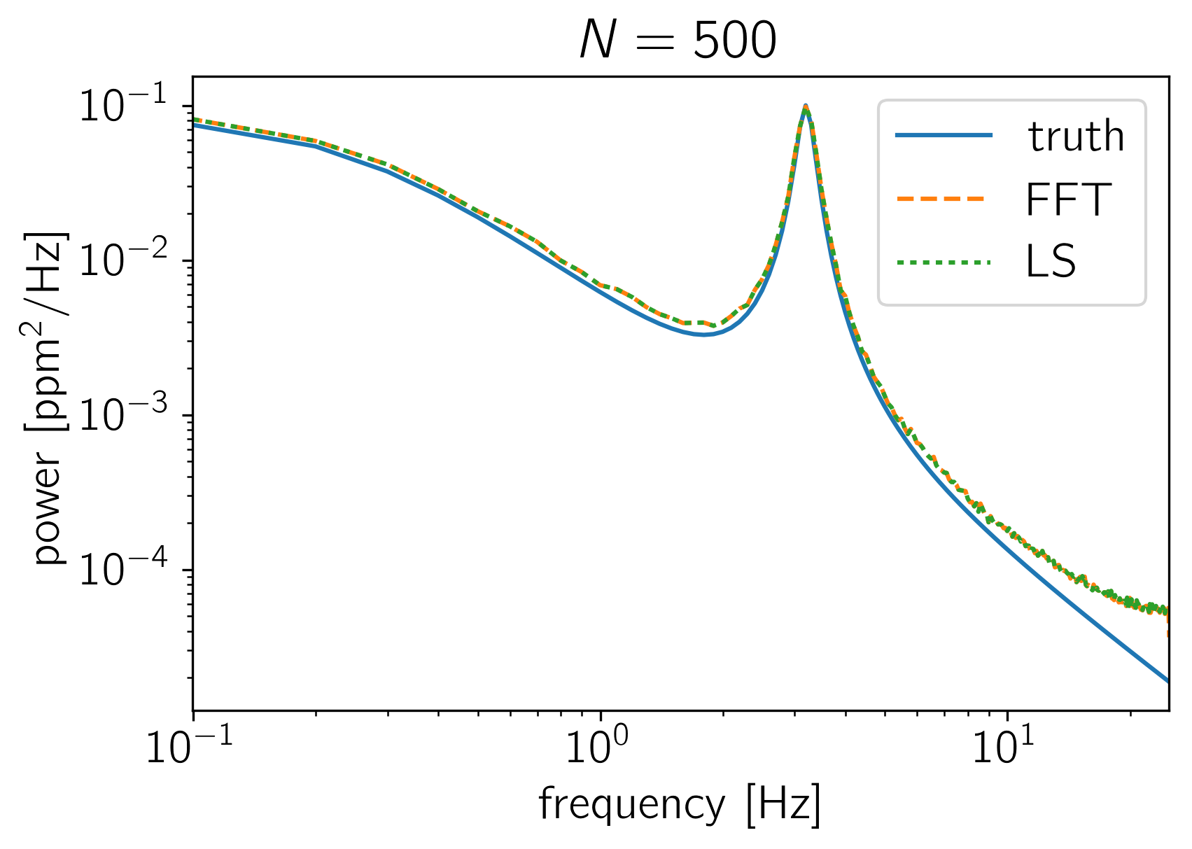
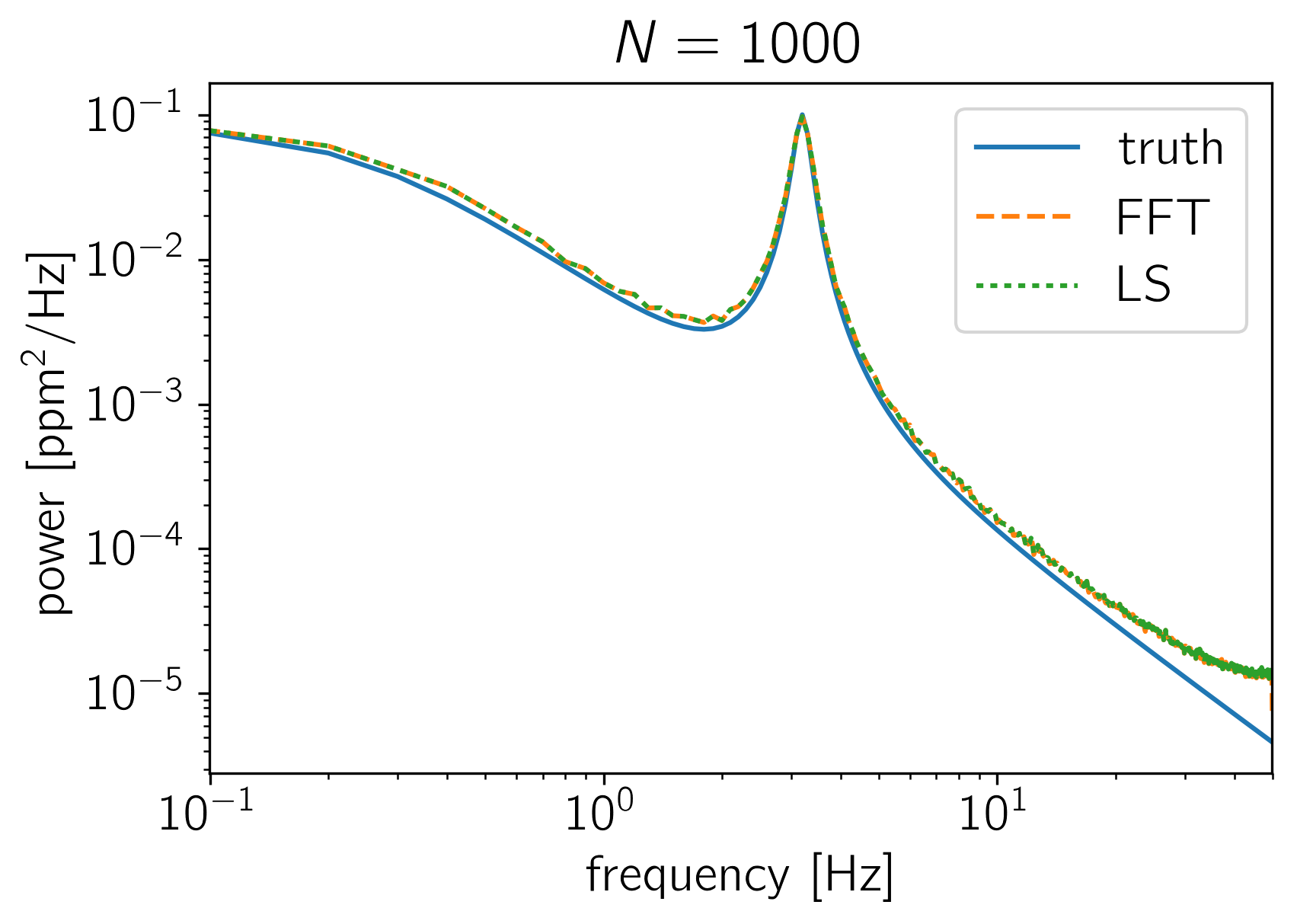
The crux of many time series analysis problems is the question of where all the factors of \(N\) and \(2\,\pi\) enter. In this tutorial, we’ll look at how the PSD returned by celerite should be compared to an estimate made using NumPy’s FFT library or to an estimate made using a Lomb-Scargle periodogram. To make this comparison, we’ll sample many realizations from a celerite GP and compute the empirical power spectrum using the standard methods and compare this (numerically) to the true power spectrum as defined by celerite.
To start, here’s a function that simulates \(K\) random datasets with \(N\) data points from a celerite model and computes the mean FFT and Lomb-Scargle estimators of the power spectrum.
import numpy as np
import matplotlib.pyplot as plt
from astropy.stats import LombScargle

import celerite
from celerite import terms

def simulate_and_compute_psds(N, K=1500):
    # Set up a simple celerite model
    kernel = terms.RealTerm(0.1, 0.5) + terms.ComplexTerm(0.5, 0.05, 3.0)
    gp = celerite.GP(kernel)

    # Simulate K datasets with N points
    t = np.linspace(0, 10, N)
    gp.compute(t)
    np.random.seed(42)
    y = gp.sample(size=K)

    # Compute the FFT based power spectrum estimates
    f = np.fft.rfftfreq(len(t), t[1] - t[0])
    fft = np.array(list(map(np.fft.rfft, y)))
    fft *= np.conj(fft)

    # >>> To get the FFT based PSD in the correct units, normalize by N^2 <<<
    power_fft = fft.real / N**2

    # Compute the LS based power spectrum estimates
    power_ls = []
    for y0 in y:
        model = LombScargle(t, y0)
        power_ls.append(model.power(f[1:-1], method="fast", normalization="psd"))
    power_ls = np.array(power_ls)

    # >>> To get the LS based PSD in the correct units, normalize by N <<<
    power_ls /= N

    # Compute the true power spectrum
    # NOTE: the 2*pi enters because celerite computes the PSD in _angular_ frequency
    power_true = kernel.get_psd(2*np.pi*f)

    # >>> To get the true PSD in units of physical frequency, normalize by 2*pi <<<
    power_true /= 2*np.pi

    # Let's plot the estimates of the PSD
    plt.figure()
    plt.plot(f, power_true, label="truth")
    plt.plot(f, np.median(power_fft, axis=0), "--", label="FFT")
    plt.plot(f[1:-1], np.median(power_ls, axis=0), ":", label="LS")
    plt.yscale("log")
    plt.xscale("log")
    plt.xlim(f.min(), f.max())
    plt.ylabel("power [$\mathrm{ppm}^2/\mathrm{Hz}$]")
    plt.xlabel("frequency [Hz]")
    plt.title("$N = {0}$".format(N))
    plt.legend()

simulate_and_compute_psds(500)
simulate_and_compute_psds(1000)
(1500, 500)
(1500, 1000)