Benchmark
To test the scaling of the celerite algorithm, the following figures show the computational cost of
gp.compute(x, yerr)
gp.log_likelihood(y)
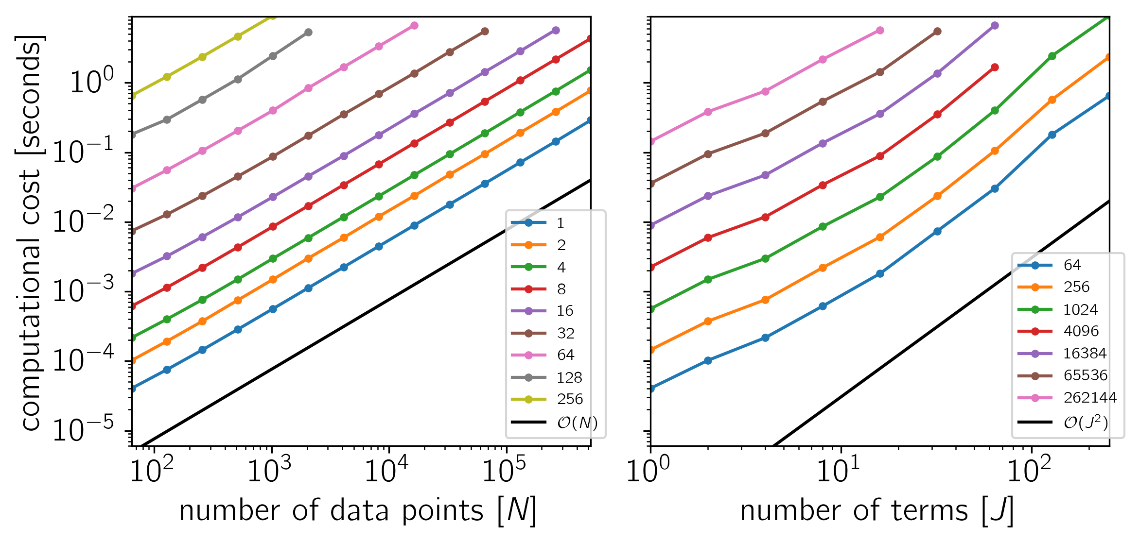
as a function of the number of data points \(N\) and the number of terms \(J\). The theoretical scaling of this algorithm should be \(\mathcal{O}(N\,J^2)\).
The code for this example is available on GitHub and below we show the results for a few different systems. In each plot, the computational time is plotted as a function of \(N\) or \(J\) and the colors correspond to the other dimension as indicated by the legend.
Example 1: On macOS with Eigen 3.3.3, pybind11 2.0.1, and NumPy 1.12.0.
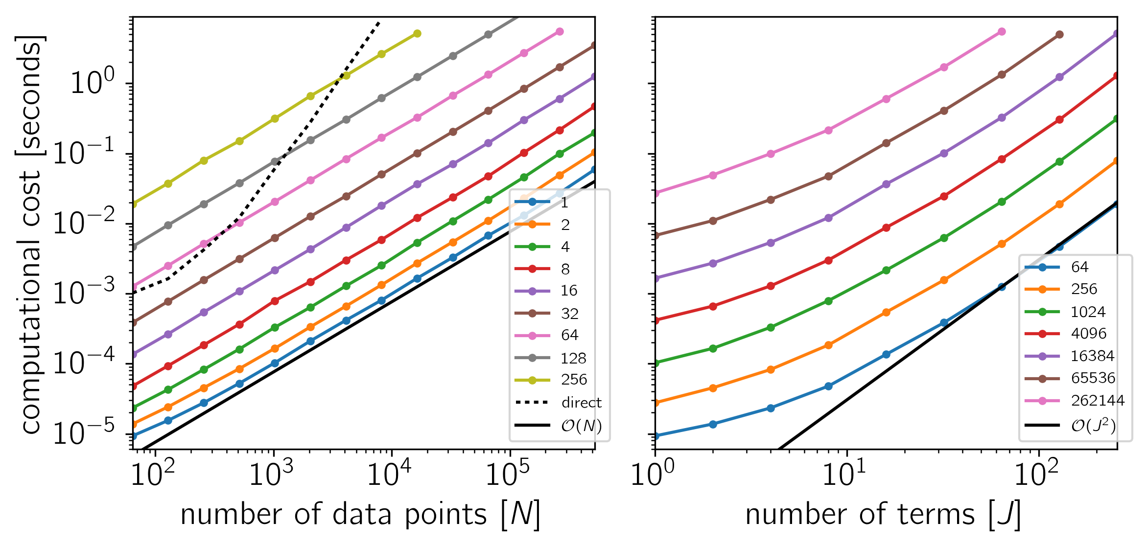
Example 2: On Linux with Eigen 3.3.3, pybind11 2.0.1, and NumPy 1.12.0.
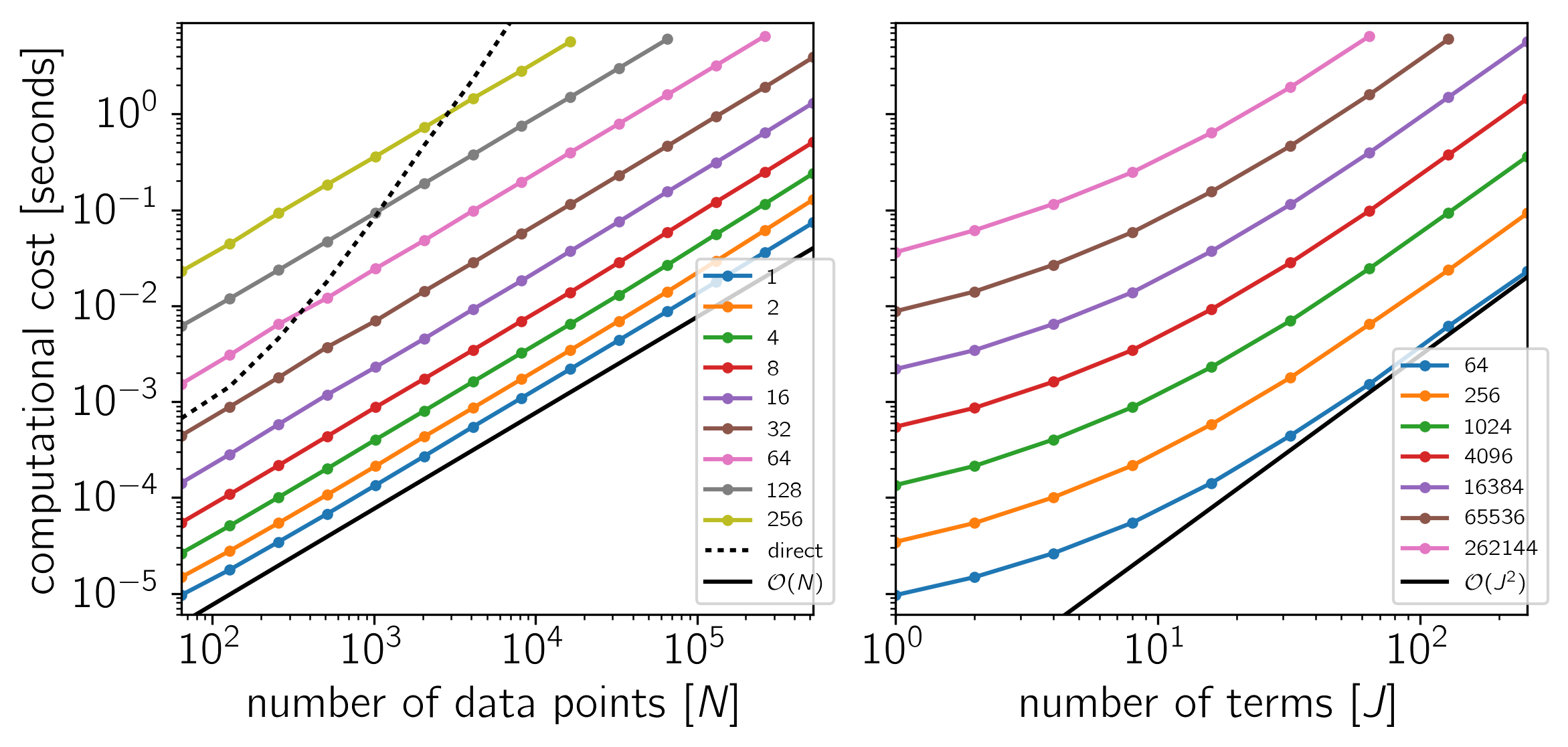
Example 3: For comparison, a CARMA solver using a Kalman filter. On Linux with Eigen 3.3.3, pybind11 2.0.1, and NumPy 1.12.0.